
In our 3-part series on "How to Assess Sensor Accuracy" this week, our CTO Paolo shares how to use R² and MAE to determine if readings from an indicative monitor are good enough to trust. If you haven't already, please read the overview here and introduction to R² here first.
Mean Absolute Error (MAE) is calculated to determine the absolute difference between the measurements of a device under analysis and the measurements of a reference instrument. It is the average of the absolute value of the deviations between measurements of the two devices. In other words, it shows how different measurements from the two devices are in value.
The MAE has the same units as the measurements, and it goes from 0 to infinity.
- A low MAE means that the measurements from the device under test are very close in absolute value to the measurements from the reference instrument.
- A high MAE means that the measurements from the device under test are very far in absolute value from the measurements from the reference instrument.
A significant difference between MAE and R² is that MAE, having the same unit as the measurement, is interpreted with knowledge of the phenomenon that we are trying to monitor.
For example, if we are measuring the weight of a human being and we are calculating MAE score for a scale, we know that a MAE of 0.5 grams is acceptable, while a MAE of 0.5 kg is not. On the other end, if we are measuring the weight of a cargo ship, a MAE of 0.5 kg is perfectly acceptable.
Covering R² Blind Spots with MAE
To see how MAE can be used to supplement the information given by R², let’s look back to the previous figures (copied below):
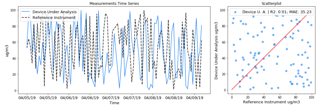

Once we calculate the R² and MAEs, we can add our knowledge of the phenomenon to the analysis. For the imaginary device that generated the top graph, no correlation with the reference instrument is observed (R² = 0.0). Furthermore, the average deviation between its measurements and the reference measurements (MAE) is 35.23 𝞵g/m3. Such deviation could lead to severe misclassification of air quality. This means that the device should be regarded as inaccurate for the purpose of monitoring ambient air quality.
For the imaginary device that generated the bottom graph, no correlation with the reference instrument is observed (R²= 0.0). However, the average deviation between its measurements and the reference measurements (MAE) is less than 2 𝞵g/m3. This means that, in principle, the device might be able to correctly classify air quality, and the low R² could be the result of a low range of pollutant concentrations during the test. In this case, it is recommended to repeat the test with a wider pollutant concentration.
One more thing to keep in mind during experimental data analysis is that the MAE metric is not a good indicator of correlated deviations that can be corrected through calibration, or deviations that are caused by random errors or limitations of the device under analysis which cannot be corrected. All kinds of deviations increase MAE equally. A device under analysis with a high R² that perfectly tracks changes in pollutant concentration, but is off by a factor potentially due to a poor calibration, might have a similar MAE to a broken device that always outputs the same number. Luckily, a high R² can point to the possibility of calibrating the device under analysis.

To avoid the pitfalls of MAE, Clarity recommends to also calculate and report R² with MAE.
If you have any additional questions about MAE or assessing sensor accuracy, please reach out to our team at contact@clarity.io.